Overview of the Slit's Diffraction Pattern
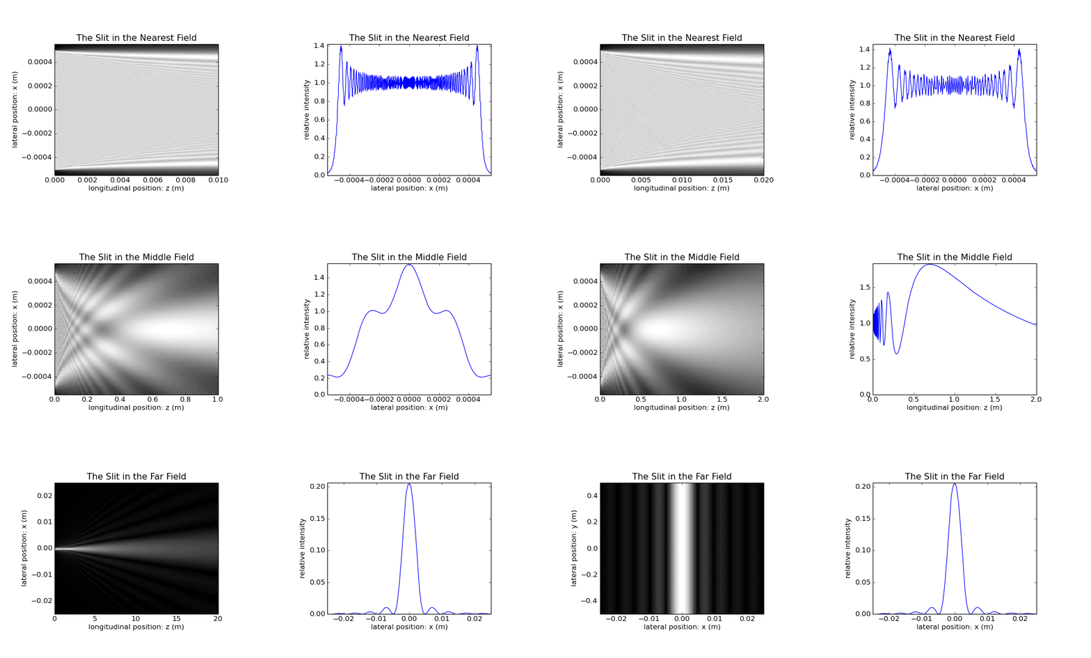
In the nearest and middle field, the transversal \(x\) scale stays invariant, and the longitudinal \(z\) scale displays more and more space. Partly there are also \(z\) profiles instead of \(x\) profiles shown.
For pictures showing an \(xz\) plot on the left and an \(x\) crosssection on the right, the lateral \(x\) profiles to the right always refer to the central \(z\) position in the diagram to the left.
In the far field, the \(x\) and \(z\) scales are choosen such that the diffraction pattern is clearly visible. On the right, first the \(z\) profile is shown, then the \(x\) profile, and finally the \(x\) profile is shown also in the 2D diagram.
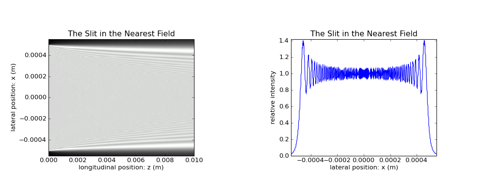
The first longitudinal centimeter behind the 1 cm wide slit.
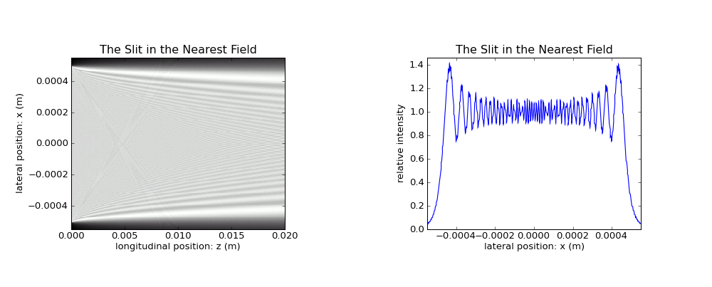
The \(z\) range increases to 2 cm.
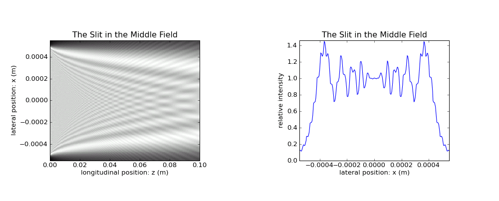
Tiny sub-lobes become clearly visible. Their structure is also shown in Sect. Central Fringes of the Slit.
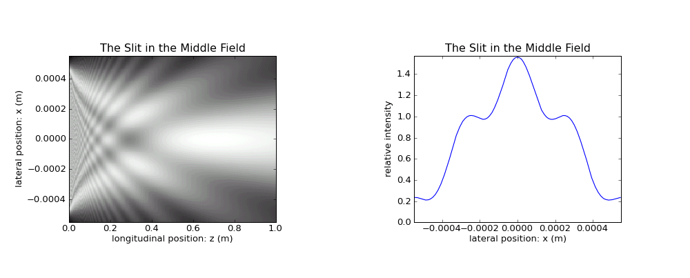
Only the most central sub-lobes survive and grow.
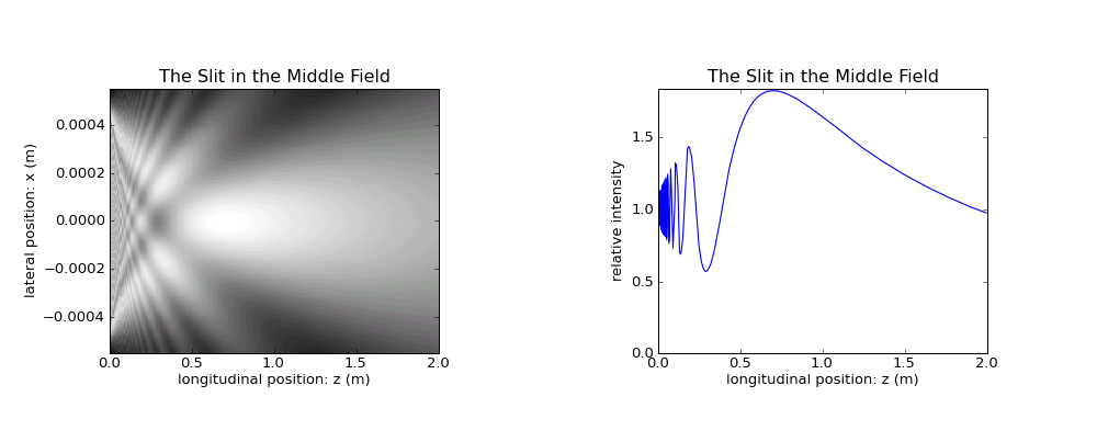
Note the transition to a \(z\) profile through central \(x\) on the right.
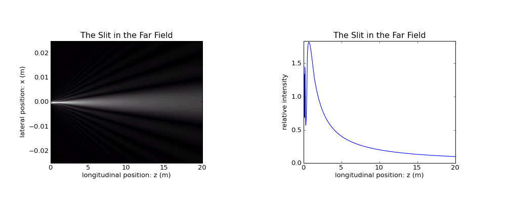
The \(x\) and \(z\) scale have been changed simultaneously.
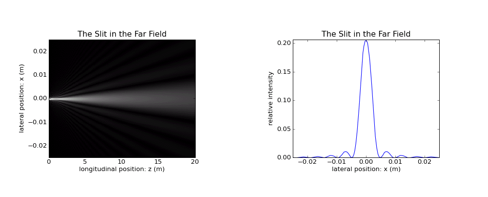
The 1D diagram shows now again an \(x\) profile at central \(z\). Note than the surviving sublobes become the final Fraunhofer diffraction pattern.
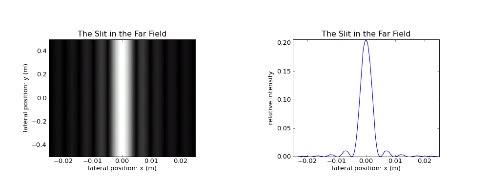
The 2D diagram too shows now the intensity profile through \(x\). Only the sublobes from the most central region are visible now as an angular pattern. None of the initial big lobes has survived except for the form factor.